参考:
PyTorch Autograd Explained-In-depth Tutoral
使用pytorch的backward()报错
使用pytorch的backward函数的时候报错:RuntimeError: grad can be implicitly created only for scalar outputs。
观察下面这段代码:
1 | import torch |
输出结果为:2.0
x是一个标量,当调用它的backward方法后会根据链式法则自动计算出叶子节点的梯度值,如果将其换成一个矩阵或者向量呢?
1 | import torch |
得到报错:RuntimeError: grad can be implicitly created only for scalar outputs
如果 Tensor 是一个标量(即它包含一个元素的数据),则不需要为 backward() 指定任何参数,但是如果它有更多的元素,则需要指定一个 gradient 参数,该参数是形状匹配的张量。
那么为了解决上面代码的问题,需要将第5行改成如下:
1 | y.backward(gradient=torch.ones_like(x)) |
输出结果如下:
1 | tensor([[2., 2., 2., 2.], |
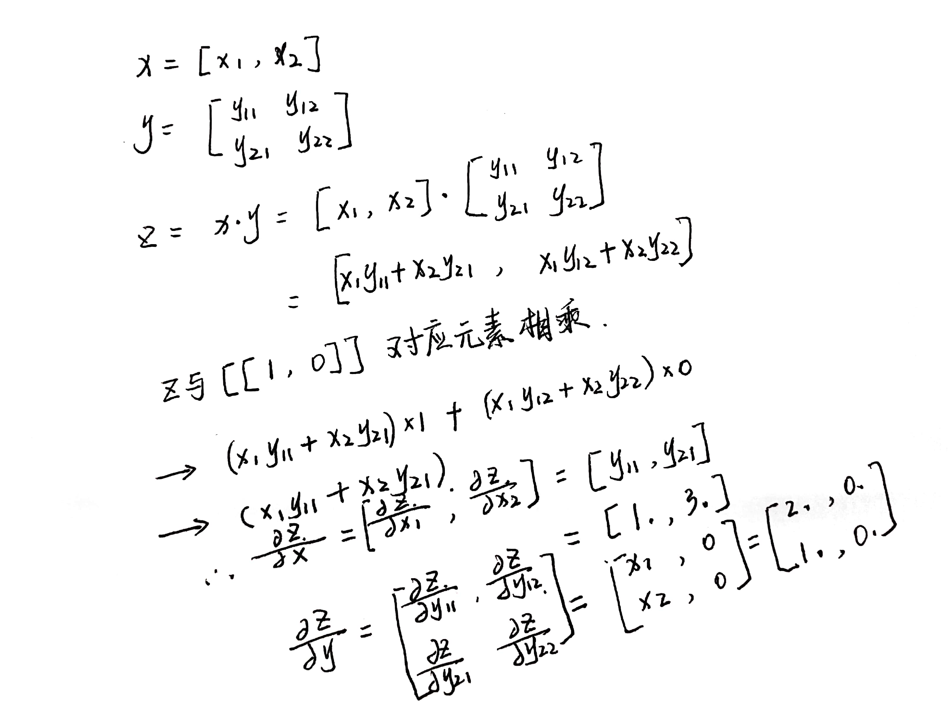
当然,最常用的是传入torch.ones_like(x)函数,也可以传入其他的张量给gradient参数,比如下面这段代码:
1 | x = torch.tensor([2., 1.], requires_grad=True) |
输出结果如下:
1 | z:tensor([[5., 8.]], grad_fn=<MmBackward>) |
z容易理解,就是两个矩阵x和y相乘的结果,反向传播的时候,计算流程如下图所示:
源代码中backward的接口定义如下:
1 | torch.autograd.backward( |
grad_tensors的作用其实可以简单地理解成在求梯度时的权重,因为可能不同值的梯度对结果影响程度不同,所以pytorch弄了个这种接口,而没有固定为全是1。
PyTorch Basics
Tensors:张量在Pytorch中相当于一个高维数组,除了可以加载到CPU,张量还可以加载到GPU从而加速计算。只要将一个张量的参数设置为:requires_grad=True,他们就会自动构建反向传播计算图,并跟踪每一次在该张量上的运算,以便于使用静态计算图(dynamic computation graph)来计算张量。
在早期版本的pytorch中,torch.autograd.Variable类被用来创建支持梯度计算和操作符跟踪的张量,但是Torch v0.4.0中Variable类已经被弃用了。现在在pytorch中,torch.Tensor和torch.autograd.Variable是同一个类,而且前者更适合用于跟踪运算符。
一个权重参数的梯度可以理解为:该权重的一个微小改变导致的损失值的改变。随后该梯度被用于更新权重。
注意,在pytorch中,只有浮点型的张量才可以计算梯度。可以使用如下的方式快速转换:
2
3
4
5
6
7
8
9
10
11
x = torch.randint(1, 5, (2, 3))
print(f"Int type x: \n{x}\n")
x = x.type_as(torch.FloatTensor(x.shape))
x.requires_grad_(True)
print(f"Float type x: \n{x}\n")
y = x ** 2
y.backward(torch.ones_like(x))
print(f"x.grad: \n{x.grad}\n")
Autograd:这个类记录了在一个gradient enabled张量上的所有运算符,并创建了一个静态计算图。这个计算图中,输入结点表示叶子节点,输出结点是根节点。梯度的计算是通过从根节点走到叶子节点,使用链式法则,将沿途上所有的梯度相乘得到最终叶子节点的梯度。
静态计算图(Dynamic Computational graph)
静态计算图由gradient enabled 张量和操作符共同偶见。数据流与在该数据流上的运算符在运行时就定义了,所以静态计算图的构建完全是自动的。一个设置requires_grad=False的简单相加操作的计算图构建如下(图片来自https://towardsdatascience.com/pytorch-autograd-understanding-the-heart-of-pytorchs-magic-2686cd94ec95):
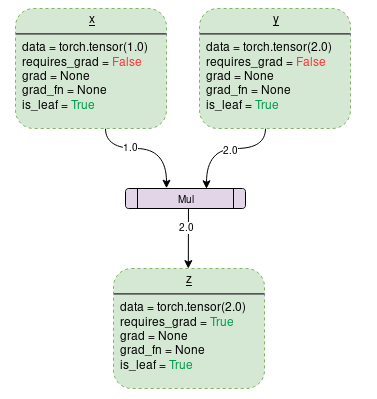
每一个虚线框表示的是图中的一个变量,紫色矩形框是一个操作符。
每一个变量都有如下的属性成员:
Data:变量的数值。
requires_grad:这个属性如果设置为True,就开始跟踪所有的操作符然后构建一个反向传播图用于计算梯度,对于任意一个张量,创建之后可以通过a.required_grad_(True)来改变其状态。
grad:这个属性表示变量的梯度值。如果requires_grad是False,那么grad值就是None,即便requires_grad是True,变量的grad属性也不能立马变成有值的状态,还需要根节点的.backward()函数操作之后才可以有梯度值。
grad_fn:该属性记录了用于计算梯度的反向传播函数。
is_leaf:如果一个节点满足以下条件之一就是叶子结点:
1. 该结点变量通过一些函数来显示初始化,比如`x=torch.tensor(1.0)`或者`x=torch.randn(1, 1)`。
2. 在对所有`requires_grad=False`的张量经过运算符操作之后创建的结点。
3. 它是通过一些张量的`.detach()`创建的。
一旦根节点执行了backward(),梯度只会被填充到requires_grad和is_leaf均为True的结点上。
如果设置requires_grad=True,pytorch会开始追踪操作符,并且将每一步的requires_grad=True的变量的梯度函数存储起来,就像下图一样(图来自https://towardsdatascience.com/pytorch-autograd-understanding-the-heart-of-pytorchs-magic-2686cd94ec95):
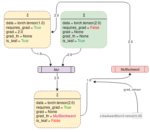
下面这段代码可以生成上述的计算图:
1 | import torch |
如果要防止pytorch追踪运算与创建反向传播图,可以将代码片段包含在with torch.no_grad():里,这可以让代码运行的更快,而且节省内存。
1 | import torch |
Jacobians and vectors
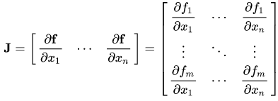
雅克比(Jacobians)矩阵:记录两个向量之间的偏导数关系。如一个向量,另一个向量,那么雅克比矩阵表示如下:
假设一个pytorch的gradient enabled张量(假设它表示的是一个机器学习模型中的权重),X经过一些操作之后得到。
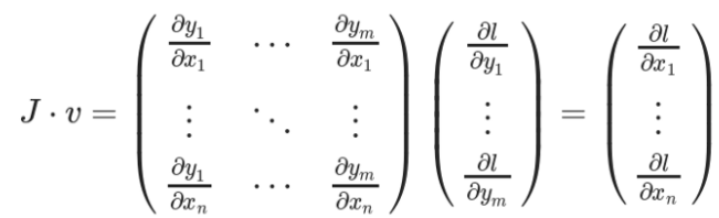
然后Y被用于计算标量损失,假设一个向量是标量损失相对于的梯度向量:
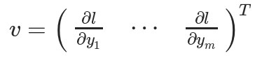
为了获得损失和权重之间的梯度,使用雅克比矩阵与相乘可以得到:
pytorch inplace operation
在pytorch中,有两种情况不能使用inplace operation:
- 对于requires_grad=True的叶子张量不能使用inplace operation;
- 对于在求梯度阶段需要用到的张量,不能使用Inplace operation。
第一种情况: requires_grad=True的leaf tensor
1 | import torch |
报错信息为:
1 | RuntimeError: a leaf Variable that requires grad is being used in an in-place operation. |
因为作为叶子结点,在设置requires_grad为True之后,计算图开始构建了,如果要在构建之后初始化权重可以这样:
1 | import torch |
第二种情况:求梯度阶段需要用到的张量
1 | import torch |
将上述代码计算图构建出来如下:
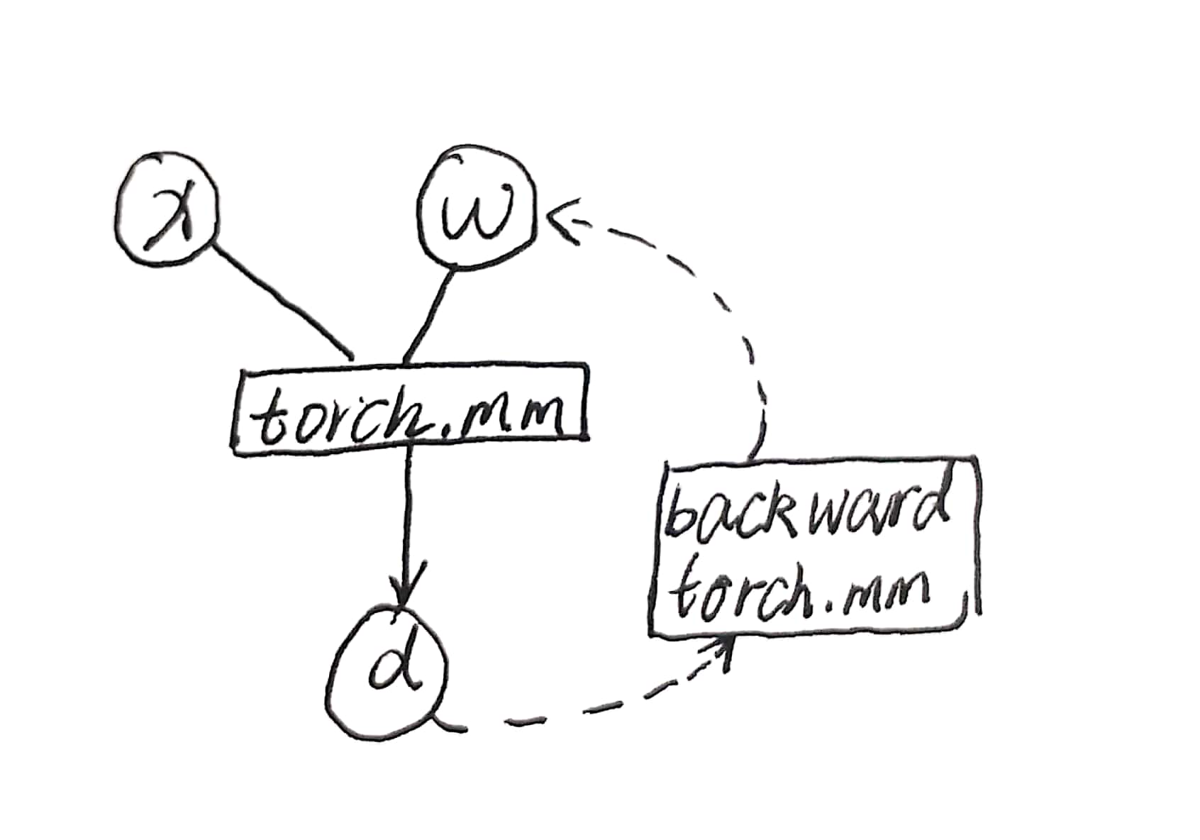
在计算得到d之后,反向求梯度的计算图就已经构建好了,而且w的梯度值的计算依赖于x的值,如果去掉代码中的注释,重新x -= 1的话,那么在反向传播的时候利用到x的值来求梯度就有误,为了防止这种错误发生,pytorch报错:
1 | RuntimeError: one of the variables needed for gradient computation has been modified by an inplace operation: |
造成错误的主要原因是,执行d=torch.mm(x, w)之后,反向求导机制保存了x的引用以便后续的反向求导计算。
x.data和x.detach()的区别
二者的相同之处在于:
- 都和x共享一块数据
- 都和x的计算历史无关
- requires_grad=False
不同之处在于,x.data在某些情况下不安全,比如上述inplace operation 的第二种情况,将上述代码修改如下:
1 | import torch |
输出结果如下:
1 | x = |
正确的w.grad应该是:
1 | tensor([[5., 5.], |
发现运算真的将原来的x数值变化了然后再求导的(这里是将x矩阵中的所有元素都减一,可以手算一下结果是符合预期的)。
上述代码中,x_和x式共享一块数据空间的,改x_就相当于改x。release note 中指出, 如果想要 detach 的效果的话, 还是 detach() 安全一些.
1 | import torch |
会有报错提示。
参考链接:
https://zhuanlan.zhihu.com/p/38475183
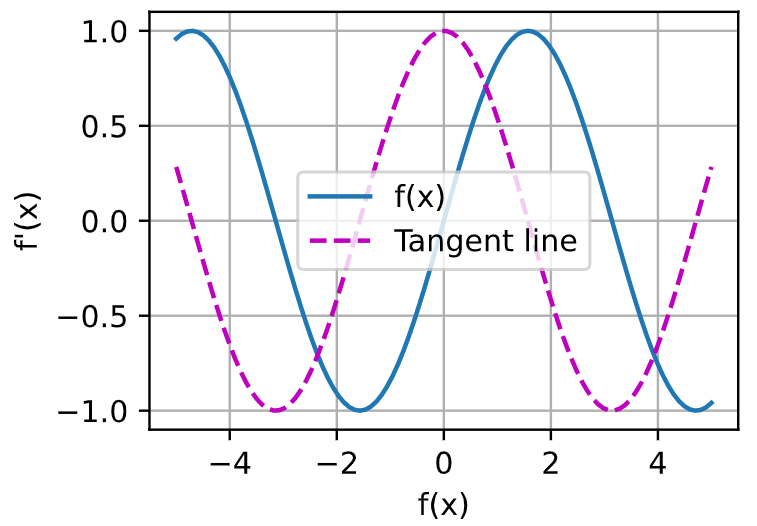
下面解决《动手学深度学习》的2.5章节的第五题:

代码如下:
1 | x = torch.linspace(-5, 5, 100) |
结果如下:
参考: